How to Track Google Adsense Check Using Payment and Tracking Number ?

IndiaHow to Track Google adsense check Position – Hello Friends we got very  excited when we reach to Our First Google adsense check (When we reach $ 100 or above for our fist Payment form Google ) Many people want to know how to Track Google adsense check position Google Our check dispatch or not and when we will receive our  check . Google also respect our Feeling and Google gives an option for Track our check status.

Follow Below step for track your check status

1st Option

Go to your adsense account and select right side on the top Finalized earnings Details » 

There you will be see last issued payment Now Click view details in payment history. By clicking this option you will be reach to bottom there you will be see your payment detail see below image as demo.

Now Copy Payment No. - Without 0 (Zero) suppose your Payment no. is 070395427 So Just Copy only 70395427.

Now Go to Blue dart Website www.bluedart.com  on website you will be see Track your Shipment Option Select Click Ref.no.  (Radio Button) and now Past your Payment No. without zero and click to Go Button Your Check Status will be Show. (See Below Image as Demo)

2nd Option

You can also Track your Check by Tracking Number (Waybill) you will find Tracking Number below of Payment No. It’s look Like this Tracking Number  BlueDart40408335155

Now Just go to blue dart website www.bluedart.com  on website you will be see Track your Shipment Option Select Click Waybill  (Radio Button) and now Past your this Tracking Number  and click to Go Button Your Check Status will be Show.


Note:-1  Adsense Take (4-10 Days ) for Upload Tracking Number . So you can use Upper given 1st option for Track your Check Status.

Note:-2 Google Dispatch our Check between 1st to 10th of month and Convert our earning in our Local Country currency between 20th to 30th of Month.

Read More

How to Convert Numbers into Words in Excel

Convert number into word in Excel you can convert numbers in spell example 1510 One Thousand Five Hundred Ten Only like this. For use this feature we need to create a function this function work in all excel version Microsoft Excel 2003, 2007, 2010, 2013,

How to convert numbers into word in excel automatically?

Follow Below step for use number to word converting function.

Open excel File Press Alt+F11 a new windows will appear (Microsoft visual basic).

Now in new window press Insert option and then Module.

Now copy below given code and past in window which opened by press Insert > module.

Function SpellNum(amt As Variant) As Variant
Dim FIGURE As Variant
Dim LENFIG As Integer
Dim i As Integer
Dim WORDs(19) As String
Dim tens(9) As String
WORDs(1) = "One"
WORDs(2) = "Two"
WORDs(3) = "Three"
WORDs(4) = "Four"
WORDs(5) = "Five"
WORDs(6) = "Six"
WORDs(7) = "Seven"
WORDs(8) = "Eight"
WORDs(9) = "Nine"
WORDs(10) = "Ten"
WORDs(11) = "Eleven"
WORDs(12) = "Twelve"
WORDs(13) = "Thirteen"
WORDs(14) = "Fourteen"
WORDs(15) = "Fifteen"
WORDs(16) = "Sixteen"
WORDs(17) = "Seventeen"
WORDs(18) = "Eighteen"
WORDs(19) = "Nineteen"
tens(2) = "Twenty"
tens(3) = "Thirty"
tens(4) = "Fourty"
tens(5) = "Fifty"
tens(6) = "Sixty"
tens(7) = "Seventy"
tens(8) = "Eighty"
tens(9) = "Ninety"
FIGURE = amt
FIGURE = Format(FIGURE, "FIXED")
FIGLEN = Len(FIGURE)
If FIGLEN < 12 Then
FIGURE = Space(12 - FIGLEN) & FIGURE
End If
If Val(Left(FIGURE, 9)) > 1 Then
SpellNum = ""
ElseIf Val(Left(FIGURE, 9)) = 1 Then
SpellNum = ""
End If
For i = 1 To 3
If Val(Left(FIGURE, 2)) < 20 And Val(Left(FIGURE, 2)) > 0 Then
SpellNum = SpellNum & WORDs(Val(Left(FIGURE, 2)))
ElseIf Val(Left(FIGURE, 2)) > 19 Then
SpellNum = SpellNum & tens(Val(Left(FIGURE, 1)))
SpellNum = SpellNum & WORDs(Val(Right(Left(FIGURE, 2), 1)))
End If
If i = 1 And Val(Left(FIGURE, 2)) > 0 Then
SpellNum = SpellNum & " Crore "
ElseIf i = 2 And Val(Left(FIGURE, 2)) > 0 Then
SpellNum = SpellNum & " Lakh "
ElseIf i = 3 And Val(Left(FIGURE, 2)) > 0 Then
SpellNum = SpellNum & " Thousand "
End If
FIGURE = Mid(FIGURE, 3)
Next i
If Val(Left(FIGURE, 1)) > 0 Then
SpellNum = SpellNum & WORDs(Val(Left(FIGURE, 1))) + " Hundred "
End If
FIGURE = Mid(FIGURE, 2)
If Val(Left(FIGURE, 2)) < 20 And Val(Left(FIGURE, 2)) > 0 Then
SpellNum = SpellNum & WORDs(Val(Left(FIGURE, 2)))
ElseIf Val(Left(FIGURE, 2)) > 19 Then
SpellNum = SpellNum & tens(Val(Left(FIGURE, 1)))
SpellNum = SpellNum & WORDs(Val(Right(Left(FIGURE, 2), 1)))
End If
FIGURE = Mid(FIGURE, 4)
If Val(FIGURE) > 0 Then
SpellNum = SpellNum & " Paise "
If Val(Left(FIGURE, 2)) < 20 And Val(Left(FIGURE, 2)) > 0 Then
SpellNum = SpellNum & WORDs(Val(Left(FIGURE, 2)))
ElseIf Val(Left(FIGURE, 2)) > 19 Then
SpellNum = SpellNum & tens(Val(Left(FIGURE, 1)))
SpellNum = SpellNum & WORDs(Val(Right(Left(FIGURE, 2), 1)))
End If
End If
FIGURE = amt
FIGURE = Format(FIGURE, "FIXED")
If Val(FIGURE) > 0 Then
SpellNum = SpellNum & " Only "
End If
End Function

After Past Code close this window.

Now come to excel sheet and save this excel sheet.

Note while saving excel sheet it will ask saving a macro free workbook Click Yes Button.

Now your excel file is ready to use for convert number to spell.

New Function Name is SpellNum.

Use Function Like this

=SpellNum(cell Address) press Enter.

Output Result

Note: If you don’t want to show Only Word in end remove this from code.

SpellNum = SpellNum & " Only " Remove this Only word from the code.

Alos Read How to count characters in excel cell

Read More

How to send thumbnail change Magic image in whatsapp

whatsapp magic image change trick send magic image to your friend’s mobile this image show as 2 type image before download it’s look different but after download it will be change you may have receive this type magic picture it’s very easy to send you only need to install a android application (.apk) in your android mobile magiapp application is most popular app for create magic image.

Magic effect Image for whatsapp Do Magic Effect.

How to create whatsapp magic effect image by magiapp.

First Install magiapp Download

>Download magiapp<

Open this app there is a two box for select two picture/image

First box image will show in chat area before download and second image will show after download.

Select two pictures after than press DoMagic button after press domagic button whatsapp will be open now select the person name whom you want to send this magic pic.

Read More

How to use Android Mobile Phone as a Modem

Use your android phone device as a modem and access mobile internet on your PC laptop system you can use your mobile internet on computer laptop or tablet device you not need to use two internet connection one in your computer and second n your mobile device use your single mobile internet on your computer use your mobile android as a modem.

How to use mobile internet on computer?

Accessing of mobile internet data on PC it’s very easy to access android mobile net in PC follow below steps for use mobile net in PC.

• Connect your mobile to computer by USB cable.
• After connect mobile with PC go to mobile setting option.

• Now click on more…Option.

• Now click on Tethering & portable hotspot option.

• Now Click on Use tethering option.

• Now wait for few second net is connecting now you computer is ready use mobile internet in PC.

Thanks I hope you like this Post.

Read More

Excel CHOOSE Function With Examples

What Does It Do?
This function picks from a list of options based upon an Index value given to by the user.

Syntax  

 =CHOOSE(UserValue, Item1, Item2, Item3 through to Item29)

Formatting

No special formatting is required.

Example  

The following table was used to calculate the medals for athletes taking part in a race.
The Time for each athlete is entered.
The =RANK() function calculates the finishing position of each athlete.
The =CHOOSE() then allocates the correct medal.
The =IF() has been used to filter out any positions above 3, as this would cause
the error of #VALUE to appear, due to the fact the =CHOOSE() has only three items in it.

Read More

Excel CHAR Function with Example

What Does It Do?
This function converts a normal number to the character it represent in the ANSI
character set used by Windows.

Syntax

 =CHAR(Number)
 The Number must be between 1 and 255.

Formatting

The result will be a character with no special formatting.

Example

The following is a list of all 255 numbers and the characters they represent.
Note that most Windows based program may not display some of the special characters,
these  will be displayed as a small box.

Note-

Number 32 does not show as it is the SPACEBAR character.

Read More

Excel CELL Function with Example

What Does It Do ?

This function examines a cell and displays information about the contents, position and formatting.

Syntax

=CELL("TypeOfInfoRequired",CellToTest)
The TypeOfInfoRequired is a text entry which must be surrounded with quotes " ".

Formatting

No special formatting is needed.

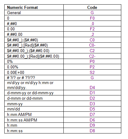
Codes used to show the formatting of the cell.

Example

The following example uses the =CELL() function as part of a formula which extracts the filename.

=MID(CELL("filename"),FIND("[",CELL("filename"))+1,FIND("]",CELL("filename"))-FIND("[",CELL("filename"))-1)

Read More

Ceiling Function in Excel With Example

What Does It Do ?

This function rounds a number up to the nearest multiple specified by the user.

Syntax

=CEILING(ValueToRound,MultipleToRoundUpTo)
The ValueToRound can be a cell address or a calculation.

Formatting

No special formatting is needed.

Example 1

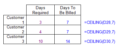
The following table was used by a estate agent renting holiday apartments.

The properties being rented are only available on a weekly basis.

When the customer supplies the number of days required in the property the =CEILING()

function rounds it up by a multiple of 7 to calculate the number of full weeks to be billed.

I

Example 2

The following table was used by a builders merchant delivering products to a construction site.

The merchant needs to hire trucks to move each product.

Each product needs a particular type of truck of a fixed capacity.

Table 1 calculates the number of trucks required by dividing the Units To Be Moved by the Capacity of the truck.
This results of the division are not whole numbers, and the builder cannot hire just part of a truck.

Table 2 shows how the =CEILING() function has been used to round up the result of the division to a whole number, and thus given the exact amount of trucks needed.

Example 3

The following tables were used by a shopkeeper to calculate the selling price of an item.

The shopkeeper buys products by the box.

The cost of the item is calculated by dividing the Box Cost by the Box Quantity.

The shopkeeper always wants the price to end in 99 pence.

Table 1 shows how just a normal division results in varying Item Costs.

Table 2 shows how the =CEILING() function has been used to raise the Item Cost to always end in 99 pence.

Explanation

=INT(E83)                   Calculates the integer part of the price.
=MOD(E83,1)            Calculates the decimal part of the price.
=CEILING(MOD(E83),0.99)          Raises the decimal to 0.99

Read More

Formulas in Excel with Brackets

Sometimes you will need to use brackets, (also known as 'braces'), in formula.

This is to ensure that the calculations are performed in the order that you need.

The need for brackets occurs when you mix plus or minus with divide or multiply.

Mathematically speaking the * and / are more important than + and - . The * and / operations will be calculated before + and - .
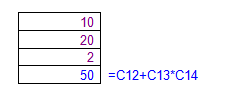
Example 1 : The wrong answer !

You may expect that 10 + 20 would equal 30
And then 30 * 2 would equal 60
But because the * is calculated first Excel sees the
calculation as 20 * 2 resulting in 40
And then 10 + 40 resulting in 50
Example 2 : The correct answer.

By placing brackets around (10+20) Excel performs this
part of the calulation first, resulting in 30
Then the 30 is multipled by 2 resulting in 60

Read More

Excel Bin2Dec Function

What Does It Do ?

This function converts a binary number to decimal.

Negative numbers are represented using two's-complement notation.

Syntax =BIN2DEC(BinaryNumber)
The binary number has a limit of ten characters.
Formatting
No special formatting is needed.

Read More

Excel Average Function Formula with Example

What Does It Do ?

This function calculates the average from a list of numbers.

If the cell is blank or contains text, the cell will not be used in the average calculation.

If the cell contains zero 0, the cell will be included in the average calculation.

Syntax

=AVERAGE(Range1,Range2,Range3... through to Range30)

Formatting

No special formatting is needed.
Note
To calculate the average of cells which contain text or blanks use =SUM() to get the total and then divide by the count of the entries using =COUNTA().

Read More

Auto SUM Shortcut key

Instead of using the AutoSum button from the toolbar, you can press Alt and = to achieve the same result.
Try it here :
Move to a blank cell in the Total row or column, then press Alt and =.
Or

Select a row, column or all cells and then press Alt and =.

Read More

Excel Formulas AND Function with Examples

What Does It Do?

This function tests two or more conditions to see if they are all true.

It can be used to test that a series of numbers meet certain conditions.

It can be used to test that a number or a date falls between an upper and lower limit.

Normally the AND() function would be used in conjunction with a function such as =IF().

Syntax

=AND(Test1,Test2)
Note that there can be up to 30 possible tests.

Formatting

When used by itself it will show TRUE or FALSE.

Example 1

The following example shows a list of examination results.

The teacher wants to find the pupils who scored above average in all three exams.

The =AND() function has been used to test that each score is above the average.

The result of TRUE is shown for pupils who have scored above average in all three exams.

Read More

Excel ABC Function with Example

What Does it Do ?

This function calculates the value of a number, irrespective of whether it is positive or negative.

Syntax

=ABS(CellAddress or Number)

Formatting

The result will be shown as a number, no special formatting is needed.

Exampe

The following table was used by a company testing a machine which cuts timber. The machine needs to cut timber to an exact length. Three pieces of timber were cut and then measured. In calculating the difference between the Required Length and the Actual Length it does not matter if the wood was cut too long or short, the measurement needs to be expressed as an absolute value.
Table 1 shows the original
calculations.
The Difference for Test 3 is shown as negative, which has a knock on effect when the Error Percentage is calculated. Whether the wood was too long or short, the percentage should still be expressed as an absolute value.

Table 2 shows the same data but using the =ABS() function to correct the calculations.

Read More